Neural Chaos
A Mathematical Biology project in collaboration with Nevaeh Ahrendsen, Jenna Ramsey-Rutledge, and Kyle Sperber.
Abstract
Neurons are fundamental units of the brain and nervous system, responsible for receiving sensory input, sending motor commands to our muscles, and transforming and relaying the electrical signals at every step in between. This project investigates neuronal dynamics using the FitzHugh-Nagumo model, exploring how different input currents influence neuronal behavior, with a focus on understanding the emergence of chaos and signal transmission in neural networks.
Biological Background
Neurons are held in an imbalanced state of ionic concentration to create a charge separation. Due to this charge separation, neurons act as electrical capacitors. The inside of the neuron increases in charge due to the movement of ions through mechanical channels until a threshold potential is reached, causing sodium channels to open. The positive sodium ions flow into the neuron increasing the voltage inside the neuron. This event is described as the action or membrane potential. Once this occurs, the signal generated propagates through the axon all the way to the terminal where the neuron releases neurotransmitters to pass along the signal and to repolarize itself. The neurotransmitters cause negative ions (typically calcium) to flow through newly opened channels to return the neuron to its resting state. During this process, the neuron can enter a refractory period where the neuron is hyperpolarized which is when the cell membrane becomes dominantly negatively charged. This behavior is demonstrated in Figure 1.
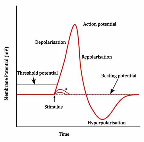
Figure 1: Neuron Behavior
Mathematical Model
From studying the neurons of a squid brain, physiologists Hodgkin and Huxley were able to derive a model that describes electrical pulses flowing through a neuron. This model consists of 4 nonlinear ordinary differential equations (ODEs). This model is shown in Figure 2 below.
Figure 2: The Hodgkin-Huxley Model
Here, $V$ is the measured action potential (Volts), and $m, h,$ and $n$ are dimensionless probabilities explaining channel subunit activation and deactivations. m represents the opening of positive sodium channels, $h$ controls the closing of the sodium channels, and n represents the potassium ion channels. While accurate, the Hodgkin-Huxley model is computationally expensive as it requires solving a system of 4 ODEs. Due to this, we chose to use the FitzHugh-Nagumo model, a simplified two-dimensional version of the Hodgkin-Huxley equations. This model relies on the facts that m can be approximated by its long-run value since it operates on a time scale an order of magnitude greater than the other variables and that the values of h and n have an approximately constant relationship allowing us to use the quasi-steady state approximation. The equations of the FitzHugh-Nagumo model are shown in Figure 3 below. We chose to use parameter values $\epsilon = 0.005$, $\alpha = 0.1$, and $\gamma = 0.5$ from the textbook Modeling Life by Garfinkel, A., Shevtsov, J., & Guo, Y.
Figure 3: The FitzHugh-Nagumo Model
Neuronal Dynamics
To initially analyze the properties of the FitzHugh-Nagumo model, the driving term $I(t)$ was converted from a time-dependent current input to a constant value $I$. This allowed for the analysis of the system to be done using the Jacobian of the FitzHugh-Nagumo Model. Through this analysis, it was found that for small values of I the system would exhibit a single stable equilibrium point. At this point, the current is insufficient to overcome the threshold potential and the neuron settles into a slightly more sensitive state without firing. This equilibrium point (EP) and its stability were found numerically and analytically. Then, as $I(t)$ increases, a Hopf Bifurcation occurs and the EP becomes unstable and the system forms a limit cycle. This corresponds to the current triggering constant firing of the neuron. Due to this, there is a positive correlation between the magnitude of $I$ and the frequency of oscillations of the membrane potential. These dynamics are demonstrated in the animated figure below. Note that for low values of $I$, solutions converge to a single value but as $I$ increases oscillations and a limit cycle emerge.
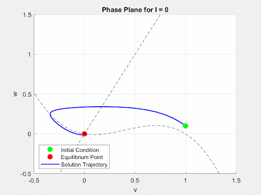
Figure 4: Autonomous Dynamics
Chaos Analysis
The FitzHugh-Nagumo model exhibits chaos as the system becomes loaded with a time-dependent input current. To push the system into chaos our group added a square wave driving current to the system. For large periods the system exhibits a limit cycle as seen in the figure below.
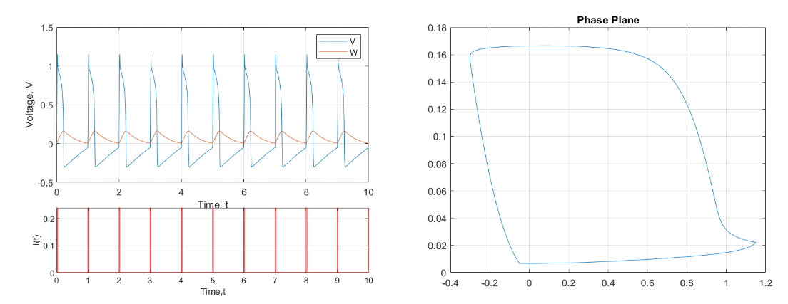
Figure 5: Limit Cycle
But, as the period of the square wave decreases the system begins to enter chaos, a deterministic but unpredictable state where small perturbations in initial conditions lead to extreme differences in solution trajectories. This is shown in the following figure.
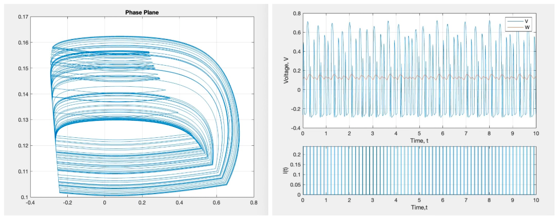
Figure 6: Chaos
Neuron Network Dynamics
After running the analysis of a singular neuron, a network of neurons was modeled by linking a series of neurons. The first neuron receives the same external driving current $I(t)$. Subsequent neurons receive a coupling current proportional to the voltage of the previous neuron, scaled by a constant resistance $R$. This simulates the transmission of signals between neurons via synapses. The resulting system of equations is,

Figure 7: Extended FitzHugh-Nagumo
When the first neuron is stimulated with a square wave with a refractory period long enough for the neuron to return to its rest state before the next pulse, the signal is transmitted through the neurons as expected. This behavior is shown in the following plot.
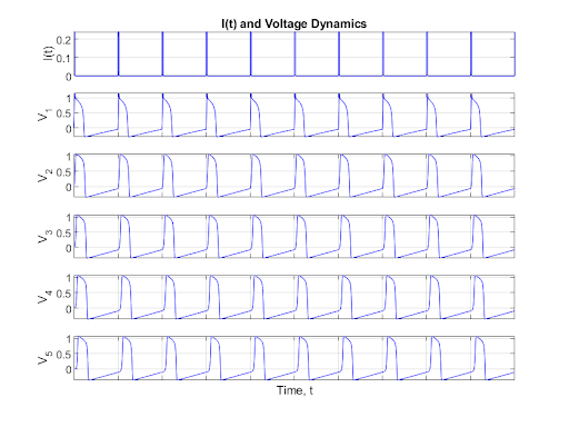
Figure 8: Regular Pulse Neuron Chain
This process illustrates that the dynamics of the first neuron have a cascading effect. For a large period, as seen above, the behavior of each of the neurons converges to a limit cycle having stable oscillations. However, as the period of the input current decreases, chaotic dynamics emerge in the first neuron. The chaos then trickles down and stabilizes through the connected neurons as shown below.
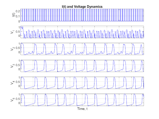
Figure 9: Quick Pulse Neuron Chain
In the above figure, it can be seen that the first neuron exhibits strong chaotic behavior, but as the signal propagates through the neurons the dynamics stabilize to a limit cycle. This is because each neuron is a capacitor that acts as a low-pass filter in linear circuit theory. This means that as the previous neuron passes in a high frequency signal the neuron filters out the high frequency noise removing some of the chaotic dynamics. This allows the system to restabilize into a limit cycle.
Conclusions
Overall it was found that for constant current input signals the FitzHugh-Nagumo model would converge to either a stable equilibrium point or a limit cycle. However, as time-dependent current input such as a square wave for high period inputs the system would remain in a limit cycle phase plane trajectory. However, as the period decreased the system began to exhibit chaotic properties propagating potentials with aperiodic structure. Then, in linking neurons to see how the chaos of a neuron is transmitted through the system, we found that the chaos settles into a limit cycle. This is likely important for the functioning of the brain as a natural self-correcting to prevent chaotic behavior and it is possible that neurological disorders may arise when neuron connections cannot correct uncontrolled chaotic oscillations.
Even though the FitzHugh-Nagumo model is a nice simplification of the Hodgkin-Huxley model that can be realistically computed, it loses information on the dynamics of the neuron since it generalizes the behaviors of ion channels in the neuron. This will lose finer details in an individual neuron and the behaviors it exhibits as well as when neurons are linked the way a chain of neurons respond to chaos may change.
Moving forward, we would like to expand this project by modeling a more sophisticated network of neurons such as having two neurons input into one neuron. We would also like to use the full Hodgkin-Huxley model and attempt to predict the behavior of one neuron under chaotic conditions to see if similar patterns arise like seen in the FitzHugh-Nagumo model. Alternatively, we could attempt to link neurons together under the Hodgkin-Huxley model to see if similar chaos smoothing occurs.
References
- Woodruff, A. (2023, October 3). What is a neuron? Queensland Brain Institute - University of Queensland. https://qbi.uq.edu.au/brain/brain-anatomy/what-neuron.
- Neuronal Activity. Neuronal Activity - an overview | ScienceDirect Topics. (n.d.). https://www.sciencedirect.com/topics/neuroscience/neuronal-activity.
- Gerstner, W., Kistler, W. M., Naud, R., & Paninski, L. (2016). Neuronal dynamics from single neurons to networks and models of cognition. Cambridge University Press.
- Purves D, Augustine GJ, Fitzpatrick D, et al., editors. Neuroscience. 2nd edition. Sunderland (MA): Sinauer Associates; 2001. Chapter 2, Electrical Signals of Nerve Cells. Available from: https://www.ncbi.nlm.nih.gov/books/NBK11053/.
- Klimenko, T. (2022, September 8). Spinal Propagation in the Neuron (Neurophysiology) | Full Discussion. YouTube. https://www.youtube.com/watch?v=r2gma7gsq6g.
- Braun, J. (2021). Hodgkin-Huxley Model. Otto-von-Guericke-Universit¨ at Magdeburg, Cognitive Biology Group Lecture 4.
- Baxter, D. A., & Byrne, J. H. (2014). Dynamical Properties of Excitable Membranes. In J. H. Byrne, R. Heidelberger, & M. N. Waxham (Eds.), From Molecules to Networks (3rd ed., pp. 409-442). Academic Press. https://doi.org/10.1016/B978-0-12-397179-1.00014-2
- Garfinkel, A., Shevtsov, J., & Guo, Y. (2017). Modeling Life. Springer eBooks. https://doi.org/10.1007/978-3-319-59731-7